Challenges With Classifying Martian Images
By Elijah Belnap, August 14, 2024
In elementary school, I used to page through picture books of images from NASA Mars rovers. I was fascinated with the idea of exploration of Mars, and even more so that the task was being done remotely through robots. Fast forward a couple of decades, and I connected my childhood fascination with Mars exploration to my more recent interest in machine learning.
The HiRise project takes high-definition images of Mars’ surface for use in scientific research. NASA published a labeled dataset of some of these images. This data set has already been cleaned and augmented for machine learning, so it’s a great data set to use for practicing machine-learning concepts.
In this post, I share my experience analyzing these HiRise images using neural networks. I’ll give an overview of my project, including some code snippets, before explaining my key takeaways from the experience. Spoiler alert: the project didn’t go quite as I imagined. I didn’t produce a useful algorithm, however, the process was valuable in introducing me to neural networks against a real data set. You can find all of my code and the necessary documentation to replicate my process on GitHub.
Why I Did This Project
To finish my bachelor’s degree, I had to perform a Capstone project. The idea was to demonstrate the skills acquired throughout the degree in a real-world scenario. I could have done a simple data analysis, however, the overachiever in me acted up and wanted to do something new. So I set out to find a machine-learning project that would stretch my current skills and force me to do new things. It turned out to be quite a bumpy ride and the project ultimately didn’t satisfy my original goals, but I did learn a lot.
With that in mind, bear with me as I’m not a subject matter expert on this topic. I also didn’t know what I was doing the whole time and had to learn during the process. The solution wasn’t an ideal fit for the task. As I mentioned earlier, I failed my original objectives. However, I think this was a great introduction to image classification and neural models for me and hopefully, it can be for others as well.
An Overview of Neural Networks
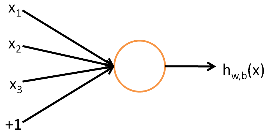
Neural networks are made up of different nodes, referred to as neurons, that each take inputs and produce outputs. I’m not going to go into depth on the mathematical side of what makes a neural network tick, as I don’t pretend to completely understand it myself, but to summarize neurons use a mathematical function to process inputs. Standford has an in-depth tutorial in which they go through the mathematical details, and you can read more here if you’re interested. The illustration below is from Standford’s article and is a simple representation of a single neuron in a neural network.

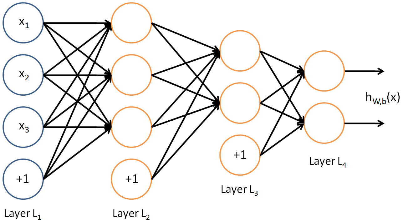
The above illustration shows various inputs into a single neuron and the output after the neuron applies its activation function. To form a multilevel neural network, multiple layers of neurons are strung together; the output of one layer becomes the input to the next layer. These layers are referred to as “hidden layers” within a model. The below diagram (also from Standford’s article) shows the first layer of inputs into the first hidden layer (L2), the output of this layer being fed to the next hidden layer as input, which feeds into the final hidden layer that produces the final output.

Like other machine-learning algorithms, these may be trained on large data sets to solve complex problems. During training, the network’s output for each gets evaluated against known “correct” outputs. The network’s function weights are then systematically adjusted based on this evaluation. The adjustment allows the network to improve its performance as training continues.
If you’d like to read more about the details of the implementation of neural networks, you can review the Standford article. If, like me, you need something that doesn’t go too far into depth on the mathematical details, I’d recommend the Wikipedia article on multilayer perception.
Code Implementation
I used Jupyter Notebooks to store and document my code. The idea was for each notebook to show a different step of the process, which started with preparing the data and ended with an evaluation of the final model. However, the majority of my notebooks focused on different training exercises to build a satisfactory model. During each training notebook, I tried tuning the values of one or more model parameters, evaluated the impact on the model, then incorporated the parameters that performed best into a model for further tuning in the next exercise.
Creating and running these notebooks took me about a month. The training exercises in particular were time-consuming, as they were computationally intensive and took anywhere from 5 to 15 hours to run on my test server. For this reason, if you wish to repeat any parts of my process I would recommend at least 12 cores and 32 GB of RAM on your test system. My system was running two Intel Xeon E5-2630 v2 processors (12 total cores), and 64 GB of RAM.
I’ll give an overview of some key parts of the code implementation before touching on my findings. The code snippets can not be run without first downloading the dataset and running my “Data Wrangling” notebook to prepare the data, but after doing that you should be able to follow along with the post.
Libraries Used
I primarily used Keras for this project, which is designed to make working with TensorFlow easier. TensorFlow is ideal for working with multidimensional arrays, or tensors. In my case, image data is represented well by tensors. Using Keras makes working with TensorFlow much more intuitive.
I occasionally used helper functions from a module I wrote for facilitating working with files, which relied on the dill library for serialization/deserialization of Python objects. This was primarily used to pass objects between notebooks for reuse.
The imports below will allow you to follow along with the other code snippet examples. However, you’ll also want to be sure to install all these libraries. The easiest way to do so may be to clone my GitHub project and set up an Anaconda environment.
import tensorflow as tf
from tensorflow import keras
from tensorflow.keras import layers
from tensorflow.keras.models import Sequential
from file_helpers import unpickle_from_file
Read the Data
If you follow my download instructions and run the Data Wrangling notebook, all the data-related files will be organized in the data directory. The /data/processed_data directory contains all the processed data we’ll need, while the ` training_images` subdirectory contains a subset of images for training. First, we’ll load a list of the assigned image labels, then we’ll load the images themselves.
The list of labels is a Python list that’s been serialized using dill. We saved this serialization to test_labels_sorted.bin in the Data Wrangling notebook. The unpickle_from_file from my file_helpers module facilitates the deserialization. Let’s deserialize the list into the labels variable.
#Import the labels for the test data set for validation purposes
labels = unpickle_from_file('../data/processed_data/test_labels_sorted.bin')
Once we have the labels, we’re ready to load the images themselves. The image_dataset_from_directory method creates a TensorFlow Dataset object from a directory path. This object doesn’t necessarily load all the images into memory immediately but rather serves as an abstraction of the data set that streams things into memory as needed. This greatly facilitates working with large data sets. However, we’ll adjust settings to prefer keeping as much of the data as we can in memory as possible.
In addition to the directory of our data set, image_dataset_from_directory takes several parameters to build out the Dataset. The validation_split parameter is how much of our data we plan to use for validation and how much we’ll want to train the model on. In our case, we’re choosing to set aside 15% of the data set for validation. The subset parameter is used to tell the method whether to load this data set as the training portion or the validation portion of the data set. The seed is the seed to use for pseudo-random functions, and I’ve chosen 123 as a seed to maintain consistency between subsequent runs. The image_size is the image dimensions of each image. The batch_size tells the model how many images to process per batch, and adjusting this parameter will affect both the processing speed and the way the model classifies the data.
The last parameter, labels, is the known labels assigned to each image. This argument expects an ordered Python list. The list should be ordered alphanumerically based on the image’s file name, as this will allow each image to be matched to the correct label.
#Read training data
batch_size = 75
img_height = 227
img_width = 227

train_ds = tf.keras.utils.image_dataset_from_directory(
  '../data/processed_data/training_images',
  validation_split=0.15,
  subset="training",
  seed=123,
  image_size=(img_height, img_width),
  batch_size=batch_size,
 labels = train_labels_sorted)

#Read validation data
val_ds = tf.keras.utils.image_dataset_from_directory(
  '../data/processed_data/training_images',
  validation_split=0.15,
  subset="validation",
  seed=123,
  image_size=(img_height, img_width),
  batch_size=batch_size,
 labels = train_labels_sorted)
Build the Model
Keras greatly simplifies building a TensorFlow model. One way it can do this is by allowing us to build the model in layers. Each layer contains a different step of the workflow, and the output of one layer is the input for the following one. Each layer may have a different function in the process.
The first layer in this model uses the rescaling method to convert input images to grayscale. The next layer (Conv2D) applies a convolution matrix to filter the image down to essential features analysis (you can read more about how this layer works here). The MaxPooling2D further simplifies the image and reduces its dimensions. I recommend A Gentle Introduction to Pooling Layers for Convolutional Neural Networks for more reading on pooling layers.
Following these layers, I’ve added a dropout layer. Neural networks tend to overfit data, so adding a dropout randomly discards some results to allow it to generalize better. This may seem counterintuitive at first, but a dropout layer placed between hidden layers can often make a model more versatile. I recommend this Dropout Regularization in Deep Learning Models with Keras article to learn more on the topic.
Flatten comes next in the model, which as the name implies flattens the dimensions of the input vectors. This prepares them to be passed to several Dense layers. The Dense layers define different neural layers in our network. In this case, we’re using layers of 256 neurons, except for the last layer which uses only one neuron for each classification class. That is because the shape of the final output will have an output prediction for each class.
img_height = 227
mg_width = 227

num_classes = 8

model_layers = [
	layers.Rescaling(1./255, input_shape=(img_height, img_width, 3)),
	layers.Conv2D(16, 3, padding='same', activation='relu'),
	layers.MaxPooling2D(),
	layers.Conv2D(32, 3, padding='same', activation='relu'),
	layers.MaxPooling2D(),
	layers.Conv2D(64, 3, padding='same', activation='relu'),
	layers.MaxPooling2D(),
	layers.Dropout(0.2),
	layers.Flatten(),
	layers.Dense(256, activation='relu'),
	layers.Dense(256, activation='relu'),
	layers.Dense(256, activation='relu'),
	layers.Dense(num_classes)]

model = Sequential(model_layers)

model.compile(optimizer=keras.optimizers.Adam(learning_rate=0.01),
		loss=tf.keras.losses.SparseCategoricalCrossentropy(from_logits=True),
		metrics=['accuracy'])
Train the Model
After we’ve defined our model, we’re ready to train it. Training consists of having the model pass the training data through each layer in batches. On each pass, the model will learn the characteristics of the data. This will allow the model to make accurate predictions on similar data sets.
Even though the code is pretty simple, this is the most intensive part of the process. You can adjust the number of epochs to determine how many passes through the training data the model makes. After each pass, the model will take what it has learned up to this point and make predictions against the validation data set. The predictions are evaluated against the set’s actual labels to produce an accuracy score for the individual training epoch. While going through training exercises, it’s often helpful to plot these scores to determine the ideal number of epochs to train for and evaluate the model’s performance using different parameters.
epochs= 5

#Silence debug messages for cleaner output
os.environ['TF_CPP_MIN_LOG_LEVEL'] = '2'

history = model.fit(
  train_ds,
  validation_data = val_ds,
  epochs = epochs
)
Evaluate Performance
During training, the model’s performance is evaluated against the validation data set. However, this validation is used as feedback during the training. Because the validation data influences the model’s training, the model’s ability to perform well on the validation data set may not be representative of how the model performs on other data sets. By evaluating against a data set that hasn’t been used to train the model we can better represent how the model will perform on other data sets.
The below code loads the data set we set aside for the final model evaluation, has the model make predictions against the data set, and outputs accuracy and loss metrics for those predictions. The accuracy and loss metrics can be used in contrast with the metrics from the validation data set used during training. This gives us a higher degree of confidence in whether or not the training metrics are accurate in reflecting the model’s performance.
#Read testing data
batch_size = 75
img_height = 227
img_width = 227

test_ds = tf.keras.utils.image_dataset_from_directory(
  '../data/processed_data/testing_images',
  seed = 123,
  image_size= (img_height, img_width),
  batch_size= batch_size,
labels = labels)

#Evaluate model
model_performance = model.evaluate(test_ds, return_dict = True)
print('The model achieved ', model_performance['accuracy'], ' accuracy on the test data set.')
print('The model achieved ', model_performance['loss'], ' loss on the test set.')
Results
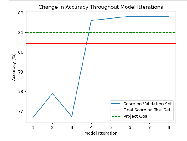
Metrics of the model’s accuracy against the validation data set were collected after each training exercise. In this way changes on the model were evaluated based on their impact on the accuracy, and changes with the highest accuracy were kept while others were discarded. The graph below shows the accuracy for each training exercise in blue, the final evaluation score in red, and the project goal accuracy as the green dotted line.
The goal was to train until the model consistently achieved over 81% accuracy. 81% was chosen as the goal because 81% of the entire dataset are images in the “other” category, which means that one could get 81% accuracy simply by labeling all images as “other”. Therefore a useful model needs to be at least more accurate than 81% to be useful.
After the fourth training exercise, further model tuning only gave marginal results. The model was achieving greater accuracy than the original goal, and although a higher accuracy would be preferred I decided that the accuracy achieved in the latest training exercises was good enough. However, on the final evaluation the model performed below the 81% goal.

What Went Wrong?
The model achieves around 80% accuracy both during training and during the final evaluation. The difference between the accuracy scores was minimal and perhaps additional tuning was needed to consistently beat the control score of 81%. However, the training exercises weren’t showing much improvement despite many attempts to optimize a variety of parameters. This had led me to incorrectly believe that perhaps the model performance was consistently good enough.
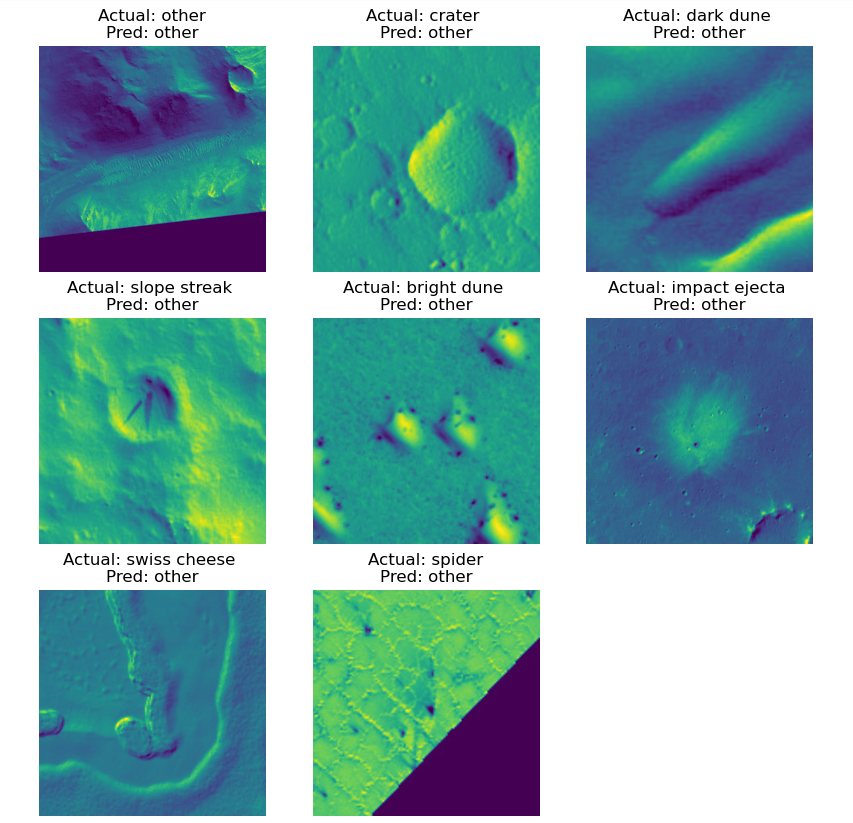
By aggregating the labels predicted by the model, the issue became clear; the model had labeled every image in the “other” catch-all category! Because the test data set was made up of around 80% of images in the “other” category, labeling them in this category allowed the model to achieve this accuracy percentage. This would also explain how the model achieved its accuracy score during training. The validation set happened to be made up of just over 81% “other” images, therefore allowing the model to achieve over 81% accuracy on the validation data set.

Lessons Learned
Classifying the HiRise images of Mars is a challenging task, especially for a beginner in neural networks such as myself. When NASA did this, they adapted a model used on Earth to classify the Martian images. I suspect this would have been much more effective and could have avoided the problem I ran into. Other things that may help would be additional parameter tuning focused on overfitting or training on a data set with a more even distribution between the image classes.
Another takeaway is to use a GPU to train the model. Unfortunately, when I performed this experiment, I didn’t have a dedicated GPU available. However, were I to repeat the experiment with a GPU training time would be greatly reduced. I’m also curious if it would have opened the doors to more complex training exercises and parameter tuning due to being able to leverage greater computing power.
Regardless, the exercise gives a good introduction to neural networks and how they work. Even though the network built in this example wasn’t effective for this problem, I’m confident that the methods learned along the way could be applied to other cases with greater success. I hope to have more opportunities to experiment with neural networks in the future and learn more about this fascinating technology.